SimPy and Salabim: A Tale of Two Simulations

Published on: June 18, 2025 by Harry Munro

When it comes to discrete-event simulation in Python, developers have a couple of excellent open-source libraries to choose from. Two prominent names are SimPy and salabim.

Recently, I shared an assembly line simulation built with SimPy. The ever-insightful Ruud van der Ham, the creator of salabim, kindly reached out with some corrections to my SimPy code and, even better, provided an equivalent model in salabim. This sparked a great opportunity to look at how these two libraries tackle the same problem.

The Scenario: A Simple Assembly Line

Our simulation models a basic assembly line with a series of stations. Parts arrive, queue for the first available station, get processed, and then move to the next station, repeating the cycle until they've passed through all stations and exit the system. We're interested in metrics like cycle time, waiting times at each station, and station utilisation.

The SimPy Approach

SimPy is a process-based discrete-event simulation framework. You define processes as Python generator functions, and these processes yield events to the simulation environment, such as timeouts or requests for shared resources.

Here's the corrected SimPy code for our assembly line:

import simpy
import random
import matplotlib.pyplot as plt
import numpy as np
import pandas as pd

RANDOM_SEED = 42
NUM_STATIONS = 3
MEAN_PROCESSING_TIMES = [5, 7, 4]
INTERARRIVAL_TIME = 3
SIMULATION_TIME = 1000
TRACE = True

part_data = []
station_busy_time = [0.0] * NUM_STATIONS
start_busy_time = [None] * NUM_STATIONS
collect_t_and_number_in_system = [(0, 0)]


def part_process(env, part_id, stations):
    if TRACE:
        print(f"{env.now:.2f}: Part {part_id} arrives at the assembly line.")
    arrival_time_system = env.now
    collect_t_and_number_in_system.append([env.now, collect_t_and_number_in_system[-1][1] + 1])

    part_details = {
        "part_id": part_id,
        "arrival_system": arrival_time_system,
        "station_entry": [None] * NUM_STATIONS,
        "service_start": [None] * NUM_STATIONS,
        "service_end": [None] * NUM_STATIONS,
        "wait_time": [None] * NUM_STATIONS,
    }
    processing_times = [random.expovariate(1.0 / MEAN_PROCESSING_TIMES[i]) for i in range(NUM_STATIONS)]
    for i in range(NUM_STATIONS):
        station = stations[i]
        part_details["station_entry"][i] = env.now
        if TRACE:
            print(f"{env.now:.2f}: Part {part_id} arrives at Station {i + 1}.")
        station_request = station.request()
        yield station_request
        part_details["service_start"][i] = env.now
        part_details["wait_time"][i] = part_details["service_start"][i] - part_details["station_entry"][i]
        if TRACE:
            print(f"{env.now:.2f}: Part {part_id} starts processing at Station {i + 1} (waited {part_details['wait_time'][i]:.2f}).")
        processing_time = processing_times[i]
        start_busy_time[i] = env.now
        yield env.timeout(processing_time)
        start_busy_time[i] = None
        part_details["service_end"][i] = env.now
        station_busy_time[i] += processing_time
        if TRACE:
            print(f"{env.now:.2f}: Part {part_id} finishes processing at Station {i + 1} (took {processing_time:.2f}).")
        station.release(station_request)
    departure_time_system = env.now
    collect_t_and_number_in_system.append([env.now, collect_t_and_number_in_system[-1][1] - 1])
    part_details["departure_system"] = departure_time_system
    part_details["cycle_time"] = departure_time_system - arrival_time_system
    if TRACE:
        print(f"{env.now:.2f}: Part {part_id} exits the assembly line. Cycle time: {part_details['cycle_time']:.2f}.")
    part_data.append(part_details)


def part_source(env, stations):
    part_id_counter = 0
    while True:
        time_to_next_arrival = random.expovariate(1.0 / INTERARRIVAL_TIME)
        yield env.timeout(time_to_next_arrival)
        part_id_counter += 1
        env.process(part_process(env, part_id_counter, stations))


print("--- Assembly Line Simulation Starting ---")
random.seed(RANDOM_SEED)
env = simpy.Environment()
stations = [simpy.Resource(env, capacity=1) for _ in range(NUM_STATIONS)]
env.process(part_source(env, stations))
env.run(until=SIMULATION_TIME)


print("--- Simulation Finished ---")
print("\n--- Simulation Results Analysis ---")
df_parts = pd.DataFrame(part_data)
if not df_parts.empty:
    avg_cycle_time = df_parts["cycle_time"].mean()
    max_cycle_time = df_parts["cycle_time"].max()
    total_parts_produced = len(df_parts)
    throughput_rate = total_parts_produced / SIMULATION_TIME
    print(f"Total parts produced: {total_parts_produced}")
    print(f"Average cycle time per part: {avg_cycle_time:.2f} minutes")
    print(f"Maximum cycle time per part: {max_cycle_time:.2f} minutes")
    print(f"Throughput rate: {throughput_rate:.2f} parts per minute")
    avg_wait_times_per_station = []
    station_utilization = []
    for i in range(NUM_STATIONS):
        valid_waits = [w for w_list in df_parts["wait_time"] if len(w_list) > i and w_list[i] is not None for w in [w_list[i]]]
        if valid_waits:
            avg_wait_times_per_station.append(np.mean(valid_waits))
        else:
            avg_wait_times_per_station.append(0)
        if start_busy_time[i]:
            station_busy_time[i] += SIMULATION_TIME - start_busy_time[i]
        utilization = (station_busy_time[i] / SIMULATION_TIME) * 100
        station_utilization.append(utilization)
        print(f"Station {i + 1} - Average Wait Time: {avg_wait_times_per_station[i]:.2f} minutes")
        print(f"Station {i + 1} - Utilization: {utilization:.2f}%")

    print("\n--- Generating Visualizations ---")
    #    plt.style.use("seaborn-v0_8-whitegrid")
    plt.figure(figsize=(10, 6))
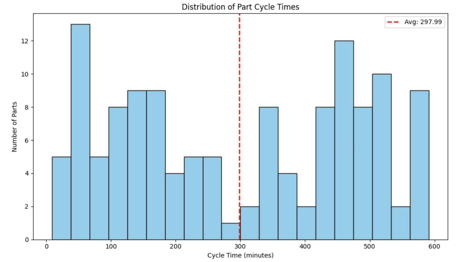
    plt.hist(df_parts["cycle_time"].dropna(), bins=20, color="skyblue", edgecolor="black")
    plt.title("Distribution of Part Cycle Times")
    plt.xlabel("Cycle Time (minutes)")
    plt.ylabel("Number of Parts")
    plt.axvline(avg_cycle_time, color="red", linestyle="dashed", linewidth=2, label=f"Avg: {avg_cycle_time:.2f}")
    plt.legend()
    plt.tight_layout()
    plt.show()

    fig, axes = plt.subplots(NUM_STATIONS, 1, figsize=(10, 4 * NUM_STATIONS), sharex=True)
    if NUM_STATIONS == 1:
        axes = [axes]
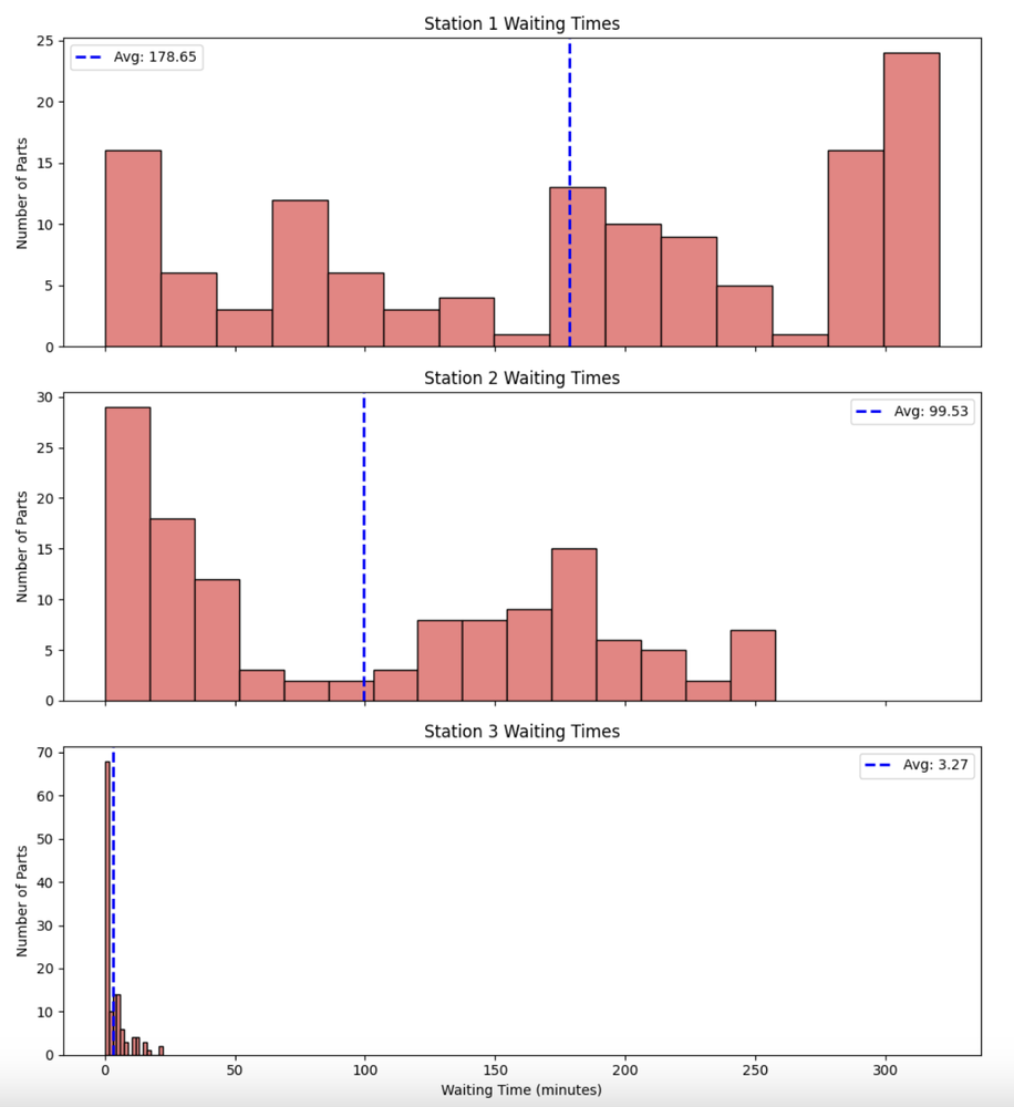
    fig.suptitle("Distribution of Waiting Times at Each Station", fontsize=16)
    for i in range(NUM_STATIONS):
        station_waits = [w_list[i] for w_list in df_parts["wait_time"] if len(w_list) > i and w_list[i] is not None]
        if station_waits:
            axes[i].hist(station_waits, bins=15, color="lightcoral", edgecolor="black")
            axes[i].set_title(f"Station {i + 1} Waiting Times")
            axes[i].set_ylabel("Number of Parts")
            avg_wait_st = avg_wait_times_per_station[i]
            axes[i].axvline(avg_wait_st, color="blue", linestyle="dashed", linewidth=2, label=f"Avg: {avg_wait_st:.2f}")
            axes[i].legend()
        else:
            axes[i].text(0.5, 0.5, "No waiting data for this station", ha="center", va="center")
            axes[i].set_title(f"Station {i + 1} Waiting Times")
    axes[-1].set_xlabel("Waiting Time (minutes)")
    plt.tight_layout(rect=[0, 0, 1, 0.96])
    plt.show()

    plt.figure(figsize=(10, 6))
    station_labels = [f"Station {i + 1}" for i in range(NUM_STATIONS)]
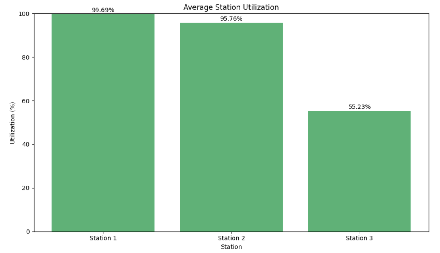
    plt.bar(station_labels, station_utilization, color="mediumseagreen")
    plt.title("Average Station Utilization")
    plt.xlabel("Station")
    plt.ylabel("Utilization (%)")
    plt.ylim(0, 100)
    for index, value in enumerate(station_utilization):
        plt.text(index, value + 1, f"{value:.2f}%", ha="center")
    plt.tight_layout()
    plt.show()

    collect_t_and_number_in_system.append((SIMULATION_TIME, collect_t_and_number_in_system[-1][1]))
    time_points, parts_in_system_count = zip(*collect_t_and_number_in_system)
    plt.figure(figsize=(12, 6))
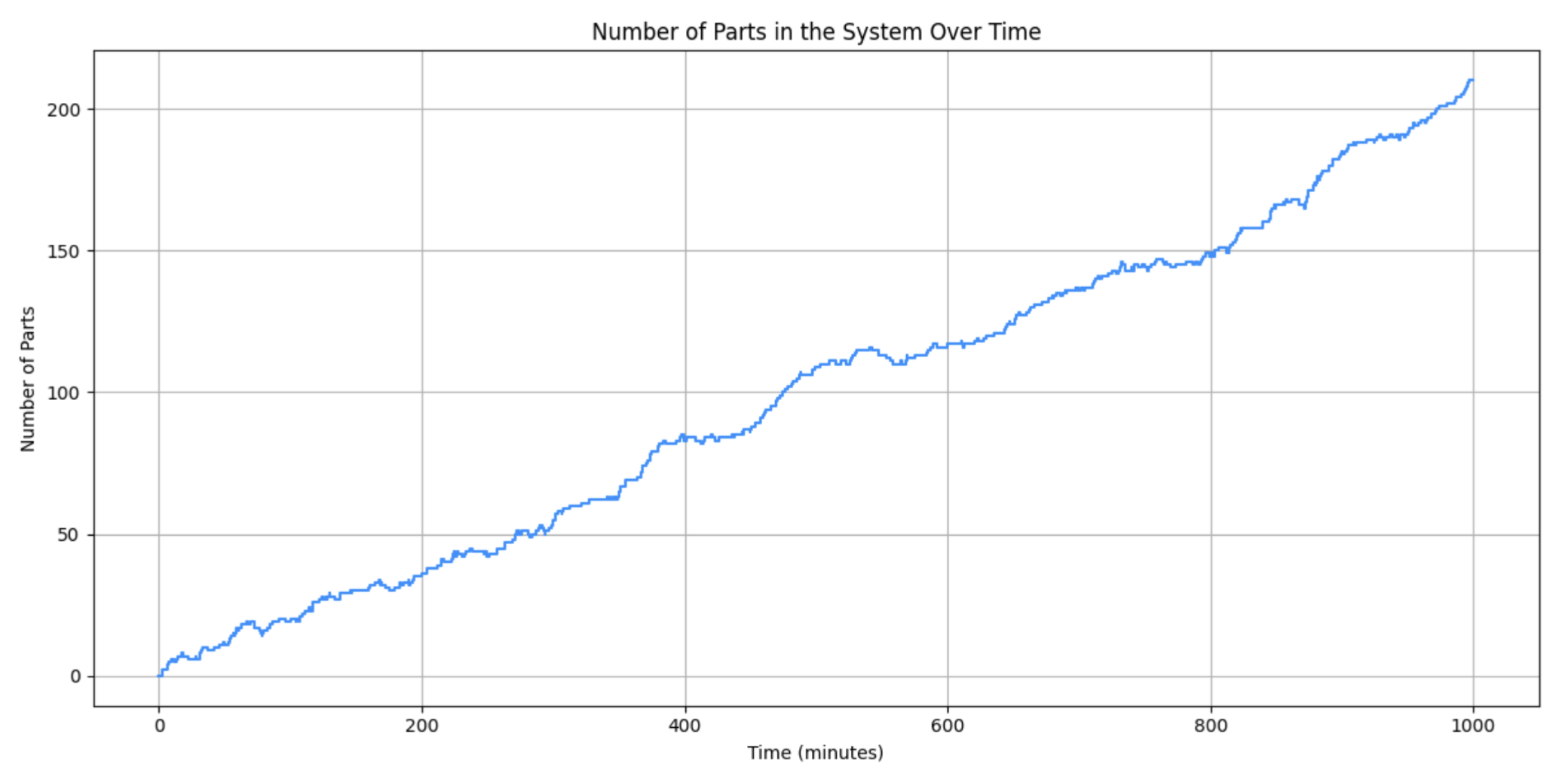
    plt.step(time_points, parts_in_system_count, where="post", color="dodgerblue")
    plt.title("Number of Parts in the System Over Time")
    plt.xlabel("Time (minutes)")
    plt.ylabel("Number of Parts")
    plt.grid(True)
    plt.tight_layout()
    plt.show()
else:
    print("No parts completed the process. Cannot generate detailed statistics or plots.")
    print("Consider increasing SIMULATION_TIME or decreasing INTERARRIVAL_TIME / MEAN_PROCESSING_TIMES.")
print("\n--- End of Script ---")
                

Key Aspects of the SimPy Code:

• Environment (simpy.Environment()): This is the core of any SimPy simulation, managing time and event scheduling.
• Resources (simpy.Resource): Each station is modelled as a Resource with a capacity of 1. This means only one part can be processed at a station at any given time.
• Processes (generator functions): part_process defines the life cycle of a part, and part_source generates new parts.
• Data Collection: Data like arrival times, service start/end times, and wait times are manually collected within part_details dictionaries and appended to the part_data list. Station busy times are tracked in station_busy_time. The number of parts in the system is tracked in collect_t_and_number_in_system.
• Analysis: After the simulation, Pandas is used to convert part_data into a DataFrame for easier calculation of statistics like average cycle time, throughput, and station-specific wait times and utilisation. Matplotlib is used for plotting.
• Randomness: Processing times and inter-arrival times are sampled from exponential distributions using Python's random module. Crucially, for a fair comparison with salabim, the processing times for all stations a part will visit are pre-sampled when the part first enters the system. This helps ensure that if both models use the same random seed, they are genuinely sampling from the same sequence of random numbers for the same events.

One important correction Ruud pointed out was in calculating station utilisation: if the simulation ends while a part is still being processed, that busy time needs to be accounted for up to SIMULATION_TIME. Similarly, tracking the number of parts in the system accurately requires recording changes as parts enter and leave, not just when they finish.

The Salabim Approach

Salabim is another Python package for discrete-event simulation. It also uses a process-oriented worldview but provides a slightly different API and some built-in features for animation and statistics collection.

Here's the salabim code for the same assembly line:

import salabim as sim
import matplotlib.pyplot as plt

sim.yieldless(False) # Allows use of 'yield' for more SimPy-like style if desired
random_seed = 42
mean_processing_time = [5, 7, 4]
interarrival_time = 3
simulation_time = 1000
animate = True
trace = False

class Station:
    def __init__(self, name, id_num): # Renamed 'id' to 'id_num'
        self._name = name
        self.resource = sim.Resource(f"{name}.resource")
        self.mon_waiting_time = sim.Monitor(f"waiting time at {name}")
        # Built-in animation for queues
        sim.AnimateQueue(self.resource.requesters(), x=900, y=700 - 100 * id_num, title=f"waiting for {name}")
        sim.AnimateQueue(self.resource.claimers(), x=1000, y=700 - 100 * id_num, title=f"{name}")

    def __repr__(self):
        return self._name

class Part(sim.Component):
    def process(self):
        self.enter(system) # Enter the overall system queue (for system count)
        
        processing_times_s = {
            station: sim.Exponential(mean_processing_time[idx]).sample() 
            for idx, station in enumerate(stations)
        }
        waiting_times_s = {}

        for station in stations:
            entry_time_station = env.now()
            yield self.request(station.resource) # Request station
            waiting_times_s[station] = env.now() - entry_time_station
            
            processing_time = processing_times_s[station]
            yield self.hold(processing_time) # Simulate processing
            self.release(station.resource) # Release station

        for station in stations:
            station.mon_waiting_time.tally(waiting_times_s[station])
        
        mon_cycle_time.tally(env.now() - self.creation_time())
        self.leave(system) # Leave the overall system queue


print("--- Assembly Line Simulation Starting ---")
env = sim.Environment(random_seed=random_seed, trace=trace, animate=animate, speed=10)

stations = [Station(name=f"station.{i}", id_num=i) for i in range(len(mean_processing_time))]

sim.ComponentGenerator(Part, iat=sim.Exponential(interarrival_time))

mon_cycle_time = sim.Monitor("cycle time")
system = sim.Queue("system") # For tracking number of parts in system

env.run(duration=simulation_time)

# --- Results Analysis (salabim) ---
print("--- Simulation Finished ---")
print("\n--- Simulation Results Analysis ---")

if mon_cycle_time.number_of_entries():
    print(f"Total parts produced: {mon_cycle_time.number_of_entries()}")
    print(f"Average cycle time per part: {mon_cycle_time.mean():.2f} minutes")
    print(f"Maximum cycle time per part: {mon_cycle_time.maximum():.2f} minutes")
    print(f"Throughput rate: {mon_cycle_time.number_of_entries() / simulation_time:.2f} parts per minute")

    for station in stations:
        print(f"{station} - Average Wait Time: {station.mon_waiting_time.mean():.2f} minutes")
        utilization = station.resource.claimed_quantity.mean() * 100 # Salabim's way
        print(f"{station} - Utilization: {utilization:.2f}%")

    print("\n--- Generating Visualizations (salabim) ---")
    
    # Distribution of Part Cycle Times
    plt.figure(figsize=(10, 6))
    plt.hist(mon_cycle_time.x(), bins=20, color="skyblue", edgecolor="black") # x() gives data points
    plt.title("Distribution of Part Cycle Times")
    plt.xlabel("Cycle Time (minutes)")
    plt.ylabel("Number of Parts")
    plt.axvline(mon_cycle_time.mean(), color="blue", linewidth=1, label=f"Mean: {mon_cycle_time.mean():.2f}")
    plt.legend()
    plt.tight_layout()
    plt.show()

    # Distribution of Waiting Times at Each Station
    fig, axes = plt.subplots(len(stations), 1, figsize=(10, 4 * len(stations)), sharex=True)
    if len(stations) == 1: axes = [axes]
    fig.suptitle("Distribution of Waiting Times at Each Station", fontsize=16)
    for i, station in enumerate(stations):
        if station.mon_waiting_time.number_of_entries():
            axes[i].hist(station.mon_waiting_time.x(), bins=15, color="lightcoral", edgecolor="black")
            axes[i].set_title(f"{station} Waiting Times")
            axes[i].set_ylabel("Number of Parts")
            mean_waiting_time = station.mon_waiting_time.mean()
            axes[i].axvline(mean_waiting_time, color="red", linewidth=1, label=f"Mean: {mean_waiting_time:.2f}")
            axes[i].legend()
        else:
            axes[i].text(0.5, 0.5, "No waiting data for this station", ha="center", va="center")
            axes[i].set_title(f"{station._name} Waiting Times") # Accessing _name directly
    axes[-1].set_xlabel("Waiting Time (minutes)")
    plt.tight_layout(rect=[0, 0, 1, 0.96])
    plt.show()

    # Average Station Utilization
    station_utilization_s = [s.resource.claimed_quantity.mean() * 100 for s in stations]
    plt.figure(figsize=(10, 6))
    station_labels_s = [f"{s}" for s in stations]
    plt.bar(station_labels_s, station_utilization_s, color="mediumseagreen")
    plt.title("Average Station Utilization")
    plt.xlabel("Station")
    plt.ylabel("Utilization (%)")
    plt.ylim(0, 100)
    for i, station in enumerate(stations): # Use enumerate to get index for text
        value = station_utilization_s[i]
        plt.text(i, value + 1, f"{value:.2f}%", ha="center")
    plt.tight_layout()
    plt.show()

    # Number of Parts in the System Over Time
    time_points_s, parts_in_system_count_s = system.length.tx() # tx() gives time and value
    plt.figure(figsize=(10, 5))
    plt.step(time_points_s, parts_in_system_count_s, where="post", color="dodgerblue")
    plt.axhline(system.length.mean(), color="blue", linewidth=1, label=f"Mean: {system.length.mean():.2f}")
    plt.title("Number of Parts in the System Over Time")
    plt.xlabel("Time (minutes)")
    plt.ylabel("Number of Parts")
    plt.legend()
    plt.grid(True)
    plt.tight_layout()
    plt.show()
else:
    print("No parts completed the process in salabim. Cannot generate detailed statistics or plots.")
print("\n--- End of Salabim Script ---")
                

Key Aspects of the salabim code:

• Environment (sim.Environment()): Similar to SimPy, this manages the simulation. Salabim's environment has built-in tracing and animation parameters.
• Component (sim.Component): Part is defined as a subclass of sim.Component. The process method here defines the part's lifecycle. salabim components manage their own process scheduling.
• Resources (sim.Resource): The Station class encapsulates a sim.Resource.
• Queues (sim.Queue): Salabim supports very powerful queues, which automatically collect statistical information in monitors.
• Monitors (sim.Monitor): Salabim has built-in Monitor objects for collecting statistics. For instance, mon_waiting_time automatically collects data tallied to it, and can then directly provide mean, max, etc., and the raw data points (.x()). station.resource.claimed_quantity is a built-in monitor for resource utilisation. system.length is a monitor for queue length.
• ComponentGenerator: Salabim offers sim.ComponentGenerator to easily create new Part components based on an inter-arrival time distribution or other conditions.
• Analysis: After the simulation, the monitors are used to present the statistics like average cycle time, throughput, and station-specific wait times and utilisation. Matplotlib is used for plotting.
• Animation (e.g. sim.AnimateQueue): Salabim provides primitives for 2D and 3D animation. AnimateQueue can visualize parts waiting for and using resources. This is a significant built-in advantage if visualization during the simulation run is important.
• sim.yieldless(False): This is here set to False. When yieldless is True (the default), salabim code can often look even more sequential, without explicit yield statements for common operations like request or hold. Setting it to False allows for a style more akin to SimPy's explicit yields.
• Randomness: sim.Exponential().sample() is one of the many distributions that salabim's supports.

Visualizing the Results

Both scripts use Matplotlib to generate similar plots:

• Histogram of part cycle times.
• Histograms of waiting times at each station.
• Bar chart of average station utilisation.
• Step plot of the number of parts in the system over time.

Because both models use the same random seed (RANDOM_SEED = 42) and the corrected logic for sampling processing times, the statistical outputs and thus the plots generated by both the SimPy and salabim versions are identical. This is a great demonstration of how, with careful attention to the random number streams, different libraries can produce the same numerical results for the same underlying model logic.

Here is the native animation of the salabim simulation:

SimPy vs. salabim: A Gentle Comparison

Both libraries are incredibly capable, yet they offer slightly different developer experiences:

• Learning Curve & Style: SimPy has a minimal API, making it feel very "Pythonic" and potentially easier to grasp initially if you're comfortable with generators. Salabim has a more extensive, object-oriented API with many built-in features, which can lead to more concise code once you're familiar with its conventions.
• Statistics Collection: SimPy is unopinionated; you build your own data collection logic, often with standard Python lists/dicts and then process it with Pandas. Salabim has powerful, built-in Monitor and Queue objects that automatically track and calculate common statistics (mean, standard deviation, length of stay, etc.), significantly reducing boilerplate code for analysis.
• Animation: This is a major differentiator. Salabim has built-in 2D (and 3D) animation capabilities. SimPy has no native animation; you would need to use external libraries and more custom code to visualize a running simulation.
• Verbosity & Features: For a simple model, SimPy can be less verbose. For more complex models, salabim's built-in features (like advanced queues, state tracking, and monitors) can make the code shorter and more declarative.
• Community & Ecosystem: SimPy has been around longer and has a larger user base, which can mean more tutorials and community examples. Salabim is very actively developed and maintained by its creator, offering excellent, direct support.

Which One Should You Choose?

Choose SimPy if:

• You prefer a minimal core library and are happy to build up statistics and visualisations using the Python ecosystem (Pandas, Matplotlib).
• You value the explicitness of Python generators for process definitions.
• You don't need built-in animation.

Choose Salabim if:

• Built-in animation is a key requirement.
• You appreciate integrated statistics collection and potentially more concise code for certain common simulation patterns, including queues and states.
• You like a more object-oriented approach.

Ultimately, both are powerful tools for discrete-event simulation in Python. The best way to decide is to try building a small model in each! Thanks again to Ruud van der Ham for the valuable input and the salabim alternative – it's collaborations like these that enrich the Python simulation community.

Looking to accelerate your simulation in Python adoption or move away from simulation software licence fees? Head over to the School of Simulation and grab your free guide to simulation in Python with SimPy.